MARGINAL COSTING
Table of content
1. INTRODUCTION
As discussed in the first chapter ‘Introduction to Cost and Management Accounting’, the cost and management accounting system, by provision of information, enables management to take various decisions. Marginal Costing is a technique of cost and management accounting which is used to analyse relationship between cost, volume and profit.
In order to appreciate the concept of marginal costing, it is necessary to study the definition of marginal costing and certain other terms associated with this technique. The important terms have been defined as follows:
1. Marginal Cost: Marginal cost as understood in economics is the incremental cost of production which arises due to one-unit increase in the production quantity. As we understood, variable costs have direct relationship with volume of output and fixed costs remains constant irrespective of volume of production. Hence, marginal cost is measured by the total variable cost attributable to one unit. For example, the total cost of producing 10 units and 11 units of a product is Rs.10,000 and Rs.10,500 respectively. The marginal cost for 11th unit i.e. 1 unit extra from 10 units is Rs.500.
Marginal cost can precisely be the sum of prime cost and variable overhead.
Example : Arnav Ltd. produces 10,000 units of product Z by incurring a total cost of Rs.3,50,000. Break-up of costs are as follows:
- Direct Material @ Rs.10 per unit, Rs.1,00,000,
- Direct employee (labour) cost @ Rs.8 per unit, Rs.80,000
- Variable overheads @ Rs.2 per unit, Rs.20,000
- Fixed overheads Rs.1,50,000 (upto a volume of 50,000 units)
In this example, if Arnav Ltd. wants to know marginal cost of producing one extra unit from the current production i.e. 10,001st unit. The marginal cost would be the change in the total cost due production of this 10,001st extra unit. The extra cost would be Rs.20, as calculated below:
| Particulars |
10,000 units |
10,001 units |
Change in Cost |
| A |
B |
C=B-A |
| Direct Material @ 10 per unit |
1,00,000 |
1,00,010 |
10 |
| Direct employee (labour) cost @ 8 per unit |
80,000 |
80,008 |
8 |
| Variable overheads @ 2 per unit |
20,000 |
20,002 |
2 |
| Fixed overheads |
1,50,000 |
1,50,000 |
0 |
| Total Cost |
3,50,000 |
3,50,020 |
20 |
2. Marginal Costing: It is a costing system where products or services and inventories are valued at variable costs only. It does not take consideration of fixed costs. This system of costing is also known as direct costing as only direct costs forms the part of product and inventory cost. Costs are classified on the basis of behavior of cost (i.e. fixed and variable) rather functions as done in absorption costing method.
3. Direct Costing: Direct costing and Marginal Costing is used synonymously at various places. But the relation of costs with respect to activity level must be understood. Some costs are variable at batch level but fixed for unit level whereas others are variable at production line level but fixed for batches and units.
Example : Arnav Ltd. produces 10,000 units of product Z by incurring a total cost of Rs.4,80,000. Break-up of costs are as follows:
- Direct Material @ Rs.10 per unit, Rs.1,00,000,
- Direct employee (labour) cost @ Rs.8 per unit, Rs.80,000
- Variable overheads @ Rs.2 per unit, Rs.20,000
- Machine set up cost @ Rs.1,200 for a production run (100 units can be manufactured in a run)
- Depreciation of a machine specifically used for production of Z Rs.10,000
- Apportioned fixed overheads Rs.1,50,000.
Analysis of the costs:
| Particulars |
10,000 units |
10,001 units |
Change in Cost |
Direct Cost |
| A |
B |
C=B-A |
| Direct Material @ 10 per unit |
1,00,000 |
1,00,010 |
10 |
Unit level direct cost |
| Direct employee (labour) cost @ 8 per unit |
80,000 |
80,008 |
8 |
Unit level direct cost |
| Varaible overheads @ 2 per unit |
20,000 |
20,0002 |
2 |
Unit level direct cost |
| Machine set up cost |
1,20,000 |
1,21,000 |
1,200 |
Batch level direct cost |
| Depreciation of a machine |
10,000 |
10,000 |
0 |
Product level direct cost |
| Apportioned fixed overheads |
1,50,000 |
1,50,000 |
0 |
Department level Direct cost |
| Total Cost |
4,80,000 |
4,81,220 |
1,220 |
|
In the example, the direct cost of producing 10,001st unit is 1,220 but it is not the marginal cost of producing one extra unit rather marginal cost of running one extra production run (batch).
4. Differential and Incremental Cost: Differential cost is difference between the costs of two different production levels. It is a relative representation of costs for two different levels that results in the increase or decrease in cost. Incremental cost, on the other hand, is the increase in the costs due to change in the volume or process of production activities. Incremental costs are sometime compared with marginal cost but in reality, there is a thin line difference between the two. Marginal cost is the change in the total cost due to production of one extra unit while incremental cost can be both for increase in one unit or in total volume. In the Example 2 above, Rs.1,220 is the incremental cost of producing one extra unit but not marginal cost for producing one extra unit.
2. CHARACTERISTICS OF MARGINAL COSTING
The technique of marginal costing is based on the distinction between product costs and period costs. Only the variables costs are treated as the costs of the products while the fixed costs are treated as period costs which will be incurred during the period regardless of the volume of output. The main characteristics of marginal costing are as follows:
- All elements of cost are classified into fixed and variable components. Semi-variable costs are also analyzed into fixed and variable elements.
- The marginal or variable costs (as direct material, direct labour and variable factory overheads) are treated as the cost of product.
- Under marginal costing, the value of finished goods and work–in–progress is also comprised only of marginal costs. Variable selling and distribution are excluded for valuing these inventories. Fixed costs are not considered for valuation of closing stock of finished goods and closing WIP.
- Fixed costs are treated as period costs and are charged to profit and loss account for the period for which they are incurred.
- Prices are determined with reference to marginal costs and contribution margin.
- Profitability of departments and products is determined with reference to their contribution margin.
3. FACTS ABOUT MARGINAL COSTING
Some of the facts about marginal costing are depicted below:
Not a distinct method: Marginal costing is not a distinct method of costing like job costing, process costing, operating costing, etc., but a special technique used for managerial decision making. Marginal costing is used to provide a basis for the interpretation of cost data to measure the profitability of different products, processes and cost centres in the course of decision making. It can, therefore, be used in conjunction with the different methods of costing such as job costing, process costing, etc., or even with other techniques such as standard costing or budgetary control.
Cost Ascertainment: In marginal costing, cost ascertainment is made on the basis of the nature of cost. It gives consideration to behaviour of costs. In other words, the technique has developed from a particular conception and expression of the nature and behaviour of costs and their effect upon the profitability of an undertaking.
Decision Making: According to traditional or total cost method, as opposed to marginal costing, the classification of costs is based on functional basis. Under this method the total cost is the sum total of the cost of direct material, direct labour, direct expenses, manufacturing overheads, administration overheads, selling and distribution overheads. In this system, other things being equal, the total cost per unit will remain constant only when the level of output or mixture is the same from period to period. Since these factors are continually fluctuating, the actual total cost will vary from one period to another. Thus, it is possible for the costing department to say one day that an item costs `20 and the next day it costs `18. This situation arises because of changes in volume of output and the peculiar 6ehavior of fixed expenses included in the total cost. Such fluctuating manufacturing activity, and consequently the variations in the total cost from period to period or even from day to day, poses a serious problem to the management in taking sound decisions. Hence, the application of marginal costing has been given wide recognition in the field of decision making.
4. DETERMINATION OF COST AND PROFIT UNDER MARGINAL COSTING
For the determination of cost of a product or service under marginal costing, costs are classified into variable and fixed. All the variable costs are part of product and services while fixed costs are charged against contribution margin.
Cost and Profit Statement under Marginal Costing
| Particulars |
Amount |
Amount |
| Revenue(A) |
|
xxx |
| Product Cost: |
|
|
| Direct Materials |
xxx |
|
| Direct employee (labour) |
xxx |
|
| Direct expenses |
xxx |
|
| Variable manufacturing overheads |
xxx |
|
| Product (Inventoriable) Costs: (B) |
xxx |
xxx |
| Product Contribution Margin {A-B} |
|
xxx |
| Variable Administration overheads |
xxx |
|
| Variable Selling & Distribution overheads |
xxx |
xxx |
| Contribution Margin: (C) |
|
xxx |
| Period Cost: (D) |
|
|
| Fixed Manufacturing expenses |
xxx |
|
| Fixed non-manufacturing expenses |
xxx |
|
| Profit/Loss {C-D} |
|
xxx |
(i) Product (Inventoriable) Costs: In the case of merchandise inventory, these are the costs which are associated with the purchase and sale of goods. In the production scenario, such costs are associated with the acquisition and conversion of materials and all other manufacturing inputs into finished product for sale. Hence, under marginal costing, variable manufacturing costs constitute inventoriable or product costs.
Finished goods are measured at product cost. Work-in-process (WIP) inventories are also measured at product cost on the basis of percentage of completion (Please refer Process & Operation costing chapter)
(ii) Contribution: Contribution or contribution margin is the difference between sales revenue and total variable costs irrespective of manufacturing or non- manufacturing.
Contribution (C) = Sales Revenue (S) - Total Variable Cost (V)
It is obtained by subtracting variable costs from sales revenue. It can also be defined as excess of sales revenue over the variable costs. The contribution concept is based on the theory that the profit and fixed expenses of a business is a ‘joint cost’ which cannot be equitably apportioned to different segments of the business. In view of this difficulty the contribution serves as a measure of efficiency of operations of various segments of the business. The contribution forms a fund for fixed expenses and profit as illustrated below:
Example:
Variable Cost = Rs.50,000, Fixed Cost = Rs.20,000,
Selling Price = Rs.80,000
Contribution = Selling Price – Variable Cost
= Rs.80,000 – Rs.50,000 = Rs.30,000
Profit = Contribution – Fixed Cost
= Rs.30,000 – Rs.20,000 = Rs.10,000
Since, contribution exceeds fixed cost; the profit is of the magnitude of Rs.10,000. Suppose the fixed cost is Rs.40,000 then the position shall be:
Contribution – Fixed cost = Profit or,
= Rs.30,000 – Rs.40,000 = - Rs.10,000
The amount of Rs.10,000 represent extent of loss since the fixed costs are more than the contribution. At the level of fixed cost of Rs.30,000, there shall be no profit and no loss.
(iii) Period Cost: These are the costs, which are not assigned to the products but are charged as expenses against the revenue of the period in which they are incurred. All fixed costs either manufacturing or non-manufacturing are recognised as period costs in marginal costing.
5. ABSORPTION COSTING
Absorption Costing is the practice of charging all costs, both variable and fixed to operations, processes or product.
In absorption costing the classification of expenses is based on functional basis whereas in marginal costing it is based on the nature of expenses. In absorption costing, the fixed expenses are distributed over products on absorption costing basis that is, based on a pre-determined level of output. Since fixed expenses are constant, such a method of recovery will lead to over or under-recovery of expenses depending on the actual output being greater or lesser than the estimate used for recovery. This difficulty will not arise in marginal costing because the contribution is used as a fund for meeting fixed expenses.
6. ADVANTAGES AND LIMITATIONS OF MARGINAL COSTING
ADVANTAGES
- Simplified Pricing Policy: The marginal cost remains constant per unit of output whereas the fixed cost remains constant in total. Since marginal cost per unit is constant from period to period within a short span of time, firm decisions on pricing policy can be taken. If fixed cost is included, the unit cost will change from day to day depending upon the volume of output. This will make decision making task difficult.
- Proper recovery of Overheads: Overheads are recovered in costing on the basis of pre-determined rates. If fixed overheads are included on the basis of pre-determined rates, there will be under- recovery of overheads if production is less or if overheads are more. There will be over- recovery of overheads if production is more than the budget or actual expenses are less than the estimate. This creates the problem of treatment of such under or over-recovery of overheads. Marginal costing avoids such under or over recovery of overheads.
- Shows Realistic Profit: Advocates of marginal costing argues that under the marginal costing technique, the stock of finished goods and work-in-progress are carried on marginal cost basis and the fixed expenses are written off to profit and loss account as period cost. This shows the true profit of the period.
- How much to produce: Marginal costing helps in the preparation of break- even analysis which shows the effect of increasing or decreasing production activity on the profitability of the company.
- More control over expenditure: Segregation of expenses as fixed and variable helps the management to exercise control over expenditure. The management can compare the actual variable expenses with the budgeted variable expenses and take corrective action through analysis of variances.
- Helps in Decision Making: Marginal costing helps the management in taking a number of business decisions like make or buy, discontinuance of a particular product, replacement of machines, etc.
- Short term profit planning: It helps in short term profit planning by B.E.P charts.
LIMITATIONS
- Difficulty in classifying fixed and variable elements: It is difficult to classify exactly the expenses into fixed and variable category. Most of the expenses are neither totally variable nor wholly fixed. For example, various amenities provided to workers may have no relation either to volume of production or time factor.
- Dependence on key factors: Contribution of a product itself is not a guide for optimum profitability unless it is linked with the key factor.
- Scope for Low Profitability: Sales staff may mistake marginal cost for total cost and sell at a price; which will result in loss or low profits. Hence, sales staff should be cautioned while giving marginal cost.
- Faulty valuation: Overheads of fixed nature cannot altogether be excluded particularly in large contracts, while valuing the work-in- progress. In order to show the correct position fixed overheads have to be included in work-in- progress.
- Unpredictable nature of Cost: Some of the assumptions regarding the behaviour of various costs are not necessarily true in a realistic situation. For example, the assumption that fixed cost will remain static throughout is not correct. Fixed cost may change from one period to another. For example, salaries bill may go up because of annual increments or due to change in pay rate etc. The variable costs do not remain constant per unit of output. There may be changes in the prices of raw materials, wage rates etc. after a certain level of output has been reached due to shortage of material, shortage of skilled labour, concessions of bulk purchases etc.
- Marginal costing ignores time factor and investment: The marginal cost of two jobs may be the same but the time taken for their completion and the cost of machines used may differ. The true cost of a job which takes longer time and uses costlier machine would be higher. This fact is not disclosed by marginal costing.
- Understating of W-I-P: Under marginal costing stocks and work in progress are understated.
7. COST-VOLUME-PROFIT (CVP) ANALYSIS
Meaning: It is a managerial tool showing the relationship between various ingredients of profit planning viz., cost, selling price and volume of activity. As the name suggests, cost volume profit (CVP) analysis is the analysis of three variables cost, volume and profit. Such an analysis explores the relationship between costs, revenue, activity levels and the resulting profit. It aims at measuring variations in cost and volume.
Assumptions:
- Changes in the levels of revenues and costs arise only because of changes in the number of product (or service) units produced and sold – for example, the number of television sets produced and sold by Sony Corporation or the number of packages delivered by Overnight Express. The number of output units is the only revenue driver and the only cost driver. Just as a cost driver is any factor that affects costs, a revenue driver is a variable, such as volume, that causally affects revenues.
- Total costs can be separated into two components; a fixed component that does not vary with output level and a variable component that changes with respect to output level. Furthermore, variable costs include both direct variable costs and indirect variable costs of a product. Similarly, fixed costs include both direct fixed costs and indirect fixed costs of a product
- When represented graphically, the behaviours of total revenues and total costs are linear (meaning they can be represented as a straight line) in relation to output level within a relevant range (and time period).
- Selling price, variable cost per unit, and total fixed costs (within a relevant range and time period) are known and constant.
- The analysis either covers a single product or assumes that the proportion of different products when multiple products are sold will remain constant as the level of total units sold changes.
- All revenues and costs can be added, subtracted, and compared without taking into account the time value of money. (Refer to the FM study material for a clear understanding of time value of money).
Importance
It provides the information about the following matters:
- The behavior of cost in relation to volume.
- Volume of production or sales, where the business will break-even.
- Sensitivity of profits due to variation in output.
- Amount of profit for a projected sales volume.
- Quantity of production and sales for a target profit level.
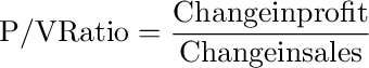
Impact of various changes on profit:
An understanding of CVP analysis is extremely useful to management in budgeting and profit planning. It elucidates the impact of the following on the net profit:
- Changes in selling prices,
- Changes in volume of sales,
- Changes in variable cost,
- Changes in fixed cost.
Marginal Cost Equation
The contribution theory explains the relationship between the variable cost and selling price. It tells us that selling price minus variable cost of the units sold is the contribution towards fixed expenses and profit. If the contribution is equal to fixed expenses, there will be no profit or loss and if it is less than fixed expenses, loss is incurred. Since the variable cost varies in direct proportion to output, therefore if the firm does not produce any unit, the loss will be there to the extent of fixed expenses. These points can be described with the help of following marginal cost equation:
Marginal Cost Equation = S -V = C = F ± P
Where,
S = Selling price per unit, V = Variable cost per unit, C = Contribution, F = Fixed Cost,
Marginal Cost Statement
| Sales |
xxxx |
| Less: Variable Cost |
(xxxx) |
| Contribution |
xxxx |
| Less: Fixed Cost |
(xxxx) |
| Profit |
xxxx |
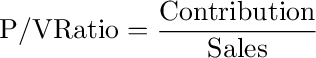
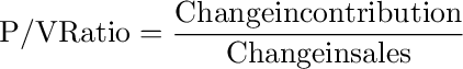
Contribution to Sales Ratio (Profit Volume Ratio or P/V ratio)
This ratio shows the proportion of sales available to cover fixed costs and profit. Contribution represent the sales revenue after deducting variable costs. This ratio is usually expressed in percentage.

A higher contribution to sales ratio implies that the rate of growth of contribution is faster than that of sales. This is because, once the breakeven point is reached, profits shall grow at a faster rate when compared to a product with a lesser contribution to sales ratio.
By transposition, we have derived the following equations:
- C = S × P/V ratio
- S = C / (P/V Ratio)
Break-Even Analysis
Break-even analysis is a generally used method to study the CVP analysis. This technique can be explained in two ways:
- In narrow sense it is concerned with computing the break-even point. At this point of production level and sales there will be no profit and loss i.e. total cost is equal to total sales revenue.
- In broad sense this technique is used to determine the possible profit/loss at any given level of production or sales.
8. METHODS OF BREAK -EVEN ANALYSIS
Break even analysis may be conducted by the following two methods:
- Algebraic computations
- Graphic presentations
(A) ALGEBRAIC CALCULATIONS
Breakeven Point
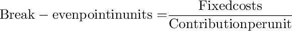
The word contribution has been given its name because of the fact that it literally contributes towards the recovery of fixed costs and the making of profits. The contribution grows along with the sales revenue till the time it just covers the fixed cost. This is the point where neither profits nor losses have been made is known as a break- even point. This implies that in order to break even the amount of contribution generated should be exactly equal to the fixed costs incurred. Hence, if we know how much contribution is generated from each unit sold we shall have sufficient information for computing the number of units to be sold in order to break even. Mathematically,
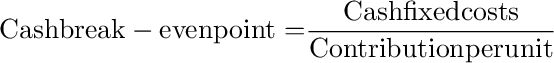
 Cash Break-even point
When break-even point is calculated only with those fixed costs which are payable in cash, such a break-even point is known as cash break-even point. This means that depreciation and other non-cash fixed costs are excluded from the fixed costs in computing cash break-even point. Its formula is –
 Multi- Product Break-even Analysis
In a multi-product environment, where more than one product is manufactured by using a common fixed cost, the break-even point formula needs some adjustments. The contribution is calculated by taking weights for the products. The weights may be of sales mix quantity or sales mix values.
(B) GRAPHICAL PRESENTATION OF BREAK EVEN CHART
Break-even Chart
A breakeven chart records costs and revenues on the vertical axis and the level of activity on the horizontal axis. The making of the breakeven chart would require you to select appropriate axes. Subsequently, you will need to mark costs/revenues on the Y axis whereas the level of activity shall be traced on the X axis. Lines representing (i) Fixed costs (horizontal line at ` 2,00,000 for ABC Ltd), (ii) Total costs at maximum level of activity (joined to the Y-axis where the Fixed cost of ` 2,00,000 is marked) and (iii) Revenue at maximum level of activity (joined to the origin) shall be drawn next.
The breakeven point is that point where the sales revenue line intersects the total cost line. Other measures like the margin of safety and profit can also be measured from the chart.
The breakeven chart for ABC Ltd (Example) is drawn below.
Contribution Breakeven chart
It is not possible to use a breakeven chart as described above to measure contribution. This is one of its major limitations especially so because contribution analysis is literally the backbone of marginal costing. To overcome such a limitation, accountants frequently resort to the making of a contribution breakeven chart which is based on the same principles as a conventional breakeven chart except for that it shows the variable cost line instead of the fixed cost line. Lines for Total cost and Sales revenue remain the same. The breakeven point and profit can be read off in the same way as with a conventional chart. However, it is also possible to read the contribution for any level of activity.
Using the same example of ABC Ltd as for the conventional chart, the total variable cost for an output of 1,700 units is 1,700 × `300 = `5,10,000. This point can be joined to the origin since the variable cost is nil at zero activity.

The contribution can be read as the difference between the sales revenue line and the variable cost line.
Profit-volume chart
This is also very similar to a breakeven chart. In this chart the vertical axis represents profits and losses and the horizontal axis is drawn at zero profit or loss.
In this chart each level of activity is taken into account and profits marked accordingly. The breakeven point is where this line interacts the horizontal axis. A profit-volume graph for our example (ABC Ltd) will be as follows,
The loss at a nil activity level is equal to Rs.2,00,000, i.e. the amount of fixed costs. The second point used to draw the line could be the calculated breakeven point or the calculated profit for sales of 1,700 units.
Advantages of the profit-volume chart
The biggest advantage of the profit-volume chart is its capability of depicting clearly the effect on profit and breakeven point of any changes in the variables. The following example illustrates this characteristic,
Example :
A manufacturing company incurs fixed costs of Rs.3,00,000 per annum. It is a single product company with annual sales budgeted to be 70,000 units at a sales price of Rs.300 per unit. Variable costs are Rs.285 per unit.
- Draw a profit volume graph, and use it to determine the breakeven point.
The company is deliberating upon an increase in the selling price of the product to Rs.350 per unit. This shall be required in order to improve the quality of the product. It is anticipated that despite increase in the selling price the sales volume shall remain unaffected, however, the fixed costs shall increase to Rs.4,50,000 per annum and the variable costs to Rs.330 per unit.
- Draw on the same graph as for part (a) a second profit volume graph and give your comments.
Solution
Figure showing changes with a profit-volume chart
Working notes (i)
The profit for sales of 70,000 units is Rs.7,50,000.
| Contribution 70,000 x (300-285) |
1,050 |
| Fixed costs |
300 |
| Profit |
750 |
This point is joined to the loss at zero activity, Rs.3,00,000 i.e., the fixed costs.
Working notes (ii)
The profit for sales of 70,000 units is Rs.9,50,000.
| Contribution 70,000 x (350-330) |
1400 |
| Fixed costs |
450 |
| Profit |
950 |
This point is joined to the loss at zero activity, Rs.4,50,000 i.e., the fixed costs.
Comments:
It is clear from the graph that there are larger profits available from option (ii). It also shows an increase in the break-even point from 20,000 units to 22,500 units, however, the increase of 2,500 units may not be considered large in view of the projected sales volume. It is also possible to see that for sales volumes above 30,000 units the profit achieved will be higher with option (ii). For sales volumes below 30,000 units option (i) will yield higher profits (or lower losses).
9. LIMITATIONS OF BREAK-EVEN ANALYSIS
The limitations of the practical applicability of breakeven analysis and breakeven charts stem mostly from the assumptions underlying CVP which have been mentioned above. Assumptions like costs behaving in a linear fashion or sales revenue remain constant at different sales levels or the stocks shall remain constant period after period are unrealistic. Similarly, the assumption that the only factor which influences costs is the ‘activity level achieved’ is erroneous because other factors like inflation also have a bearing on costs.
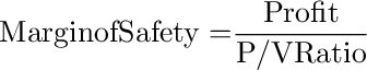
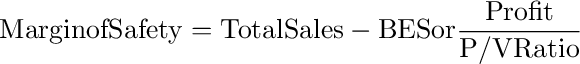
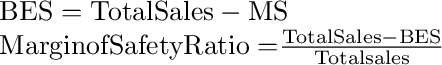
10. MARGIN OF SAFETY
The margin of safety can be defined as the difference between the expected level of sale and the breakeven sales. The larger the margin of safety, the higher is the chances of making profits. In the Example-3 if the forecast sale is 1,700 units per month, the margin of safety can be calculated as follows,
Margin of Safety = Projected sales – Breakeven sales
= 1,700 units – 1,000 units
= 700 units or 41% of sales.
The Margin of Safety can also be calculated by identifying the difference between the projected sales and breakeven sales in units multiplied by the contribution per unit. This is possible because, at the breakeven point all the fixed costs are recovered and any further contribution goes into the making of profits. It also can be calculated as:
11. VARIATIONS OF BASIC MARGINAL COST EQUATION AND OTHER FORMULAE
- Sales-Variable cost = Fixed cost±Profit/Loss
By multiplying and dividing L.H.S. by S
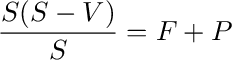

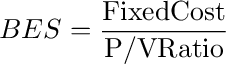
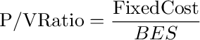
- BES*P/V Ratio=F {therefore, at BEP profit is 0}
- S*P/V Ratio = Contribution (Refer to iii.)
- (BES + MS) * P/V Ratio = Contribution (Total Sales = BES +MS)
- (BES*P/V Ratio)+(MS*P/V Ratio) = F+P
By deducting (BES × P/V Ratio) from L.H.S. and F from R.H.S. in (x) above, we get:
- MS*P/V Ratio = P
12. ANGLE OF INCIDENCE
This angle is formed by the intersection of sales line and total cost line at the break- even point. This angle shows the rate at which profit is earned once the break- even point is reached. The wider the angle the greater is the rate of earning profits. A large angle of incidence with a high margin of safety indicates extremely favourable position.
The shaded area in the graph given below is representing the angle of incidence. The angle above and below the break-even point shows the rate of earning profitability (loss). Wider angle denotes higher rate of earnings and vice-versa.

13. APPLICATION OF CVP ANALYSIS IN DECISION MAKING
As discussed earlier CVP analysis is used as an evaluation tool for managerial decisions. In this chapter we will discuss the use of CVP Analysis for short term decision making. Before going into illustration, let us discuss the decision making framework.
Framework for Decision Making
Step-1: Identification of Problem
Every organisation has its own objectives, and goals are set to achieve these objectives. To reach at the goal, actions are to be taken. For example, if an organisation wants to be a cost leader in the industry it operates in, it has to achieve 3Es in its all activities. 3Es means economy in inputs, efficiency in process and operations and effectiveness in output. An entity that exists for profit may identify few areas (problem areas) which if worked on can add to the profit or wealth maximisation. For example, Arnav Ltd. a manufacturer of Steel products, has identified that it can be leader in the industry if it can produce steel products at lower cost than its rival. Here the goal should be (problem area) low cost production.
Step- 2: Identification of Options
After identification of problem(s), the next step is identification of options to achieve the goal (to answer the problem). Every possible options need to be explored. In the above example, the Arnav Ltd. may have the following options for low cost production:
- Purchase of inputs from specialised market- Local vs Import
- Make the input in its own factory- Make or Buy
- Bulk purchase to avail discount offer- How much to purchase
- Make in-house- Make vs Outsource
- Bulk processing- How much to produce
- Using efficient machine for manufacturing- Old machine vs New machine
- Optimisation of key resources- Product mix decisions etc.
Step- 3: Evaluation of the Options
After identification of options, each option is to be evaluated against the objective criteria. An entity with objective of making profit may evaluate options on the basis of financial measures like impact of profit or loss, market share, overall impact on profitability, return on investment etc. Non-financial factors like customer satisfaction, impact on existing market/ customer, ethics of decision are also evaluated.
This step is a very important and may be grouped into two tasks
- Identification of Cost and Benefits of each options
- Estimation of amount of each options
Step-4: Selection of option:
After evaluation of the options, the best option is selected and implemented.
Principles for Identification of Cost and Benefits for measurement
The cost and benefit of an option is identified for measurement if it passes the principles of Controllability and Relevance.
- Controllability: Those cost and benefits which arise due to choice of an option. In other words, benefits received and cost incurred are directly related with the choice of the option. Thus, the costs and benefits which are controllable are considered for measurement for making decision.
- Relevance: The costs which are controllable need to be relevant for decision making. This means all controllable costs are not relevant for decision making unless it differs under the two options. Thus, a cost is treated is relevant only if (a) it is a future cost and (b) it differs under two options under consideration.
For Example, Arnav Ltd. wants to manufacture 1,000 additional units of Product X. It is considering either to manufacture in its own factory or to outsource to job workers. In this example cost of raw materials to manufacture additional 1,000 units is controllable as it arises due to management’s decision to make additional units. But it is not relevant for making choice between manufacturing in-house and outsource to job workers, as under the both options, the raw materials cost would be same.
Hence, for decision making purpose only those cost and benefits are identified for measurement which are both Controllable and Relevant.
Below is an analysis of few costs for its relevance:
| Cost |
Relevance |
Reason |
| Historical Cost |
Irrelevant |
The cost has already been incurred and do not affect the decision. Example: Book value of machinery etc. |
| Sunk Cost |
Irrelevant |
The cost which are already paid either for goods or services availed or to be availed. Example: Raw material purchased and held in store without having replacement cost, Cost of drawing, blueprint etc. |
| Committed Cost |
Irrelevant |
The committed costs are the pre-agreed cost which cannot be revoked under the normal circumstances. This is also a sunk cost. Examples: Cost of materials as per rate agreement, Salary cost to employees etc. |
| Opportunity Cost |
Relevant |
The opportunity cost is represented by the forgone potential benefit from the best rejected course of action. Had the option under consideration not chosen, the benefit would come to the organisation. |
| Notional or Imputed Cost |
Relevant |
Notional costs are relevant for the decision making only if company is actually forgoing benefits by employing its resources to alternative course of action. For example, notional interest on internally generated fund is treated as relevant notional cost only if company could earn interest from it. |
| Shut-down Cost |
Relevant |
When an organization suspends its manufacturing operations, certain fixed expenses can be avoided and certain extra fixed expenses may be incurred depending upon the nature of the industry. By closing down the manufacturing, the organization will save variable cost of production as well as some discretionary fixed costs. This particular discretionary cost is known as shut-down cost. |
Principles of Estimation of Costs and Benefits
After identification of the costs and benefits, it is now required to be quantified i.e. the cost and benefit should be measured and estimated. The estimation is done by following the two principles as discusses below:
- Variability: Variability means by how much a cost or benefit increased or decreased due to the choice of the option. Variable costs are the cost which differs under the different volume or activities. On the other hand, fixed costs remain same irrespective of volume and activities.
- Traceability: Traceability of cost means degree of relationship between the cost and the choice of the option. Direct costs are directly assigned to the option on the other hand indirect costs needs to be apportioned to the option on some reasonable basis.
For Example, Arnav Ltd. wants to manufacture 1,000 units of Product X. It is considering to manufacture the same in its own factory. To manufacture in its own factory it requires 1,000 hours of employees and a specialised machine. In this example, employee cost for labour of 1,000 hours is variable cost for in-house manufacturing and it is directly traceable. Cost of machinery is also direct cost but so far as traceability of the machinery cost is concerned it is direct cost for 1,000 units as a whole but indirect cost for a unit.
Hence, the cost and benefits of an option is measured at directly traceable and variable costs.
Short-term Decision Making using concepts of CVP Analysis
Management uses marginal costing and CVP concepts for making various decisions. In this chapter we will learn how the concepts of marginal costing and CVP is applied for analysis of identified options for short-term decision making. Generally, short-term decisions are related with temporary gaps between demand and supply for available resources. The areas of short term decision may be classified into two broad categories:
(i) Decisions related with excess supply, such as:
- Processing of Special Order
- Determination of price for stimulating demand
- Local vs Export sale
- Determination of minimum price for price quotations
- Shut-down or continue decision etc.
(ii) Decisions related with excess demand, such as:
- Make or Buy/ In-house-processing vs Outsourcing
- Product mix decision under resource constraints (limiting factors)
- Sales mix decisions
- Sale or further processing etc.
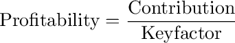
What is a Limiting Factor?
Limiting factor is anything which limits the activity of an entity. The factor is a key to determine the level of sale and production, thus it is also known as Key factor. From the supply side the limiting factor may either be Men (employees), Materials (raw material or supplies), Machine (capacity), or Money (availability of fund or budget) and from demand side it may be demand for the product, other factors like nature of product, regulatory and environmental requirement etc. The management, while making decisions, has objective to optimise the key resources upto maximum possible extent.
14. DISTINCTION BETWEEN MARGINAL AND ABSORPTION COSTING
The distinctions in these two techniques are illustrated by the following diagrams:
 Absorption Costing Approach
Marginal Costing Approach
The main points of distinction between marginal costing and absorption costing are as below:
| Marginal Costing |
Absorption Costing |
| Only variable costs are considered for product costing and inventory valuation. |
Both fixed and variable costs are considered for product costing and inventory valuation. |
| Fixed costs are regarded as period costs. The Profitability of different products is judged by their P/V ratio. |
Fixed costs are charged to the cost of production. Each product bears a reasonable share of fixed cost and thus the profitability of a product is influenced by the apportionment of fixed costs. |
| Cost data presented highlight the total contribution of each product. |
Cost data are presented in conventional pattern. Net profit of each product is determined after subtracting fixed cost along with their variable costs. |
| The difference in the magnitude of opening stock and closing stock does not affect the unit cost of production. |
The difference in the magnitude of opening stock and closing stock affects the unit cost of production due to the impact of related fixed cost. |
| In case of marginal costing the cost per unit remains the same, irrespective of the production as it is valued at variable cost. |
In case of absorption costing the cost per unit reduces, as the production increases as it is fixed cost which reduces, whereas, the variable cost remains the same per unit. |
Difference in profit under Marginal and Absorption costing
The above two approaches will compute the different profit because of the difference in the stock valuation. This difference is explained as follows in different circumstances.
-
No opening and closing stock: In this case, profit / loss under absorption and marginal costing will be equal.
-
When opening stock is equal to closing stock: In this case, profit / loss under two approaches will be equal provided the fixed cost element in both the stocks is same amount.
-
When closing stock is more than opening stock: In other words, when production during a period is more than sales, then profit as per absorption approach will be more than that by marginal approach. The reason behind this difference is that a part of fixed overhead included in closing stock value is carried forward to next accounting period.
-
When opening stock is more than the closing stock: In other words, when production is less than the sales, profit shown by marginal costing will be more than that shown by absorption costing. This is because a part of fixed cost from the preceding period is added to the current year’s cost of goods sold in the form of opening stock.


